LLM decoding is serial and memory-bandwidth bound: each pass through the model typically produces just one token. Generating several tokens at once could make much better use of GPU compute, but parallel approaches such as diffusion language models struggle to capture interactions between tokens at sampling time. Techniques that restore these interactions often drift back towards autoregressive decoding, limiting their speedups.

DSpark addresses this by pairing a parallel backbone with a lightweight autoregressive bigram model. But what if we went further and modelled the joint distribution of multiple tokens directly?

The obvious obstacle is size: a joint vocabulary grows exponentially with the number of tokens. In this post, we explore how tensor trains can make that distribution tractable—and how to normalize, train, and sample from it.

Predicting Entire Sentences at a time

In order to predict a token we first map each token to a vector, and then we take the final hidden state of a model and we find which token vector the hidden state is closest to. This requires a tensor (sometimes called the language modelling head), of size $H \times V$
where $H$ is the size of the final hidden dimension, and $V$ is the number of tokens we have, the vocabulary size.

If we wanted to jointly predict $C$ tokens at the same time this would require a vocabulary size of $V^C$.²

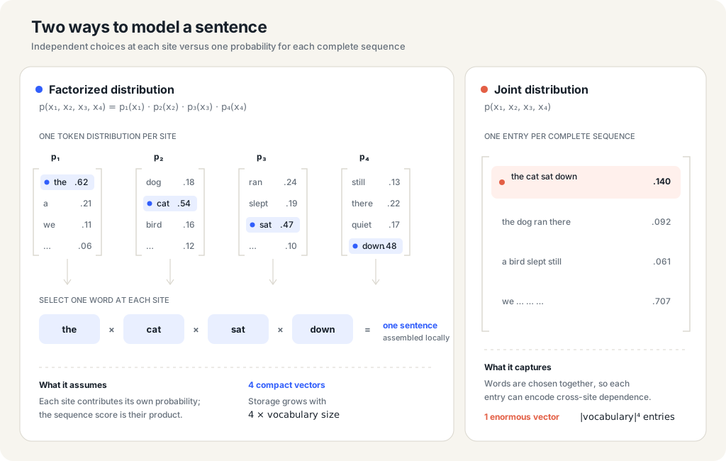
To put the ridiculousness of this in context, for a hidden size of $4096$, a vocabulary size of $256,000$ and a canvas size of $8$, with bf16 numbers, this would require approximately $1\times10^{38} GB$ of memory just to store. This is about $10^{26}$ times larger than all the data stored in S3.

Tackling the Memory Issue With Tensor Networks

Thankfully there is a scientific field that has been plagued by exponentially large matrices like this for a long time and has developed some clever tricks that could be useful here.

Quantum physics has the exact same exponential problem.³

One solution is in the field of Tensor Networks, which studies way to decompose large tensors into much smaller tensors that capture essential properties of the larger tensor. The most famous such decomposition is the SVD.⁴

This insanely large language modelling head can be decomposed into a Matrix Product State, or Tensor Train. This turns the exponential dependence on the canvas size into a linear one. Storing the tensor train language modelling head now requires $O(VCD^2)$ memory where $D$ is a hyperparameter that controls the amount of compression.

It is always possible to find a series of $M_i$ such that

$$W^{[H,V,V,V,V]} = M_1^{[H,V,D]}@M_2^{[D,V,D]}@M_3^{[D,V,D]}@M_4^{[D,V]}$$

where I have included the shapes of the tensors in the square brackets. This can be losses, if $D$ is large enough, and by choosing a small $D$ you can get substantial compression making this a workable scheme.

Shown as a tensor network here is the decomposition:

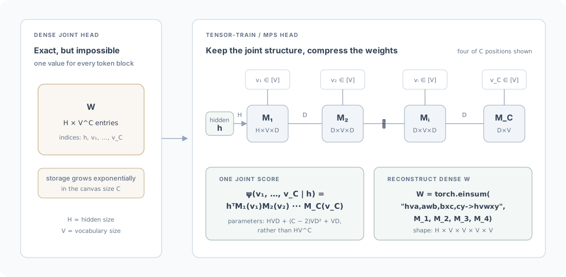
For each token site, $i$, in the canvas, we have a matrix, $M_i(v_i)$, for each vocabulary entry $v_i$. $v_i$ is just a number, the token id, and it indexes into the very large $V\times D \times D$ tensor that we store for each site in the canvas. Once the model supplies a hidden vector $h$, the contraction is the scalar amplitude

$$\psi(v_1,\ldots,v_C\mid h) = h^{\mathsf T}M_1(v_1)M_2(v_2)\cdots M_C(v_C).$$

To train this with a cross entropy loss, we need to extract the probability of a particular entry in this very large vocabulary. This requires two steps - the score of a particular set of tokens, and then the sum of the scores for all tokens to normalize and turn the score into a probability.⁵

$$p(v_1,\ldots,v_C \mid h) = \frac{|\psi(v_1,\ldots,v_C \mid h)|^2}{Z(h)}.$$

For a target block $y=(y_1,\ldots,y_C)$, the negative log-likelihood is

$$-\log p(y\mid h) = -2\log|\psi(y_1,\ldots,y_C\mid h)|+\log Z(h).$$

Training therefore needs two contractions: the target amplitude $\psi(y\mid h)$ and the global normalizer

$$Z(h)=\sum_{v_1,\ldots,v_C}|\psi(v_1,\ldots,v_C\mid h)|^2.$$

Here we present the Tensor Network Diagrams for both these terms. These diagrams are equivalent to an einsum expression which is included in the figures.

Normalization factor:

← Previous

Step 1 of 5 · Contract h, hᵀ, M₁, and M₁ᵀ

Next →

Target score:

← Previous

Step 1 of 6 · Contract h with the y₁ slice

Next →

With these two expressions we can calculate the value $p(y_1,...,y_C | h)$ which is all we need for usual cross entropy training.

How do we sample from the joint?

Sampling from this language model head isn’t completely straightforward. It follows the algorithm Sampling from an MPS / TT and translates every step into our $h,M_i,\psi,Z$ notation. In the MPS literature it is called direct sampling or perfect sampling; primary treatments include Ferris and Vidal’s perfect sampler and Han et al.’s MPS Born machine. “Perfect” does not mean that a finite-rank MPS models the data perfectly. It means that every completed block is a direct draw from the represented distribution.

A four-token perfect sample

We will work with $C=4$ as we have done above. The same recursion works for any canvas size. The chain rule factors the desired joint as

$$\begin{aligned} p(v_1,v_2,v_3,v_4\mid h) ={}&p(v_1\mid h) p(v_2\mid v_1,h)\\ &\cdot p(v_3\mid v_1,v_2,h) p(v_4\mid v_1,v_2,v_3,h). \end{aligned}$$

The linked MPS procedure obtains these four factors recursively:

1. Marginalize the other three sites. Leave the first vocabulary leg open in the doubled network and join and sum the legs at sites 2–4:

   $$p(v_1\mid h) = \frac{ \sum_{v_2,v_3,v_4}|\psi(v_1,v_2,v_3,v_4\mid h)|^2 }{Z(h)}.$$

   These $V$ values are the diagonal of what quantum physicists call the one-site reduced density matrix; the off-diagonal entries are not needed.

2. Draw the first token. Sample one value $\hat v_1$ from that $V$-way categorical distribution.

3. Project and renormalize. Contract the vocabulary leg with the one-hot basis vector $e_{\hat v_1}$, which simply selects the slice $M_1(\hat v_1)$. The surviving $D$-dimensional bond vector remembers the result of the first draw. The unnormalized mass of this branch is

   $$\sum_{v_2,v_3,v_4} |\psi(\hat v_1,v_2,v_3,v_4\mid h)|^2 =Z(h)p(\hat v_1\mid h),$$

   so divide the remaining amplitude by its square root. Equivalently, first divide the whole MPS by $\sqrt{Z(h)}$ and then divide this branch by $\sqrt{p(\hat v_1\mid h)}$, which is the convention shown in the step-by-step diagram and the linked procedure. This is the MPS version of projecting a quantum state onto the observed token and renormalizing it.

4. Recurse on the shorter train. Absorb that normalized bond vector into $M_2$. The remaining state now has three sites, and its first marginal is

   $$p(v_2\mid\hat v_1,h) = \frac{ \sum_{v_3,v_4}|\psi(\hat v_1,v_2,v_3,v_4\mid h)|^2 }{ \sum_{u=1}^{V}\sum_{v_3,v_4} |\psi(\hat v_1,u,v_3,v_4\mid h)|^2 }.$$

After drawing $\hat v_2$, repeat for sites 3 and 4. The state becomes shorter after every projection: four sites, then three, two, and one. A fresh sample restarts from $h$ and the original four-core train, so this is direct sampling rather than a Markov chain.

← Previous

Step 1 of 4 · Sample “New” at site 1

Next →

What is interesting here is that, similar to DSpark, we have found ourselves with an inherently sequential operation - to do perfect sampling you need to sample site by site and use the sample to update the information of the later steps - exactly as DSpark does! What you do gain is perhaps some expressivity in the sequential language model that you are using. This might be overkill for speculators, but there is every chance that the idea of a massively parallel backbone + lightweight sequential head for sampling takes over as the dominant language modelling paradigm since it works so well for speculators. In that case maybe this joint distribution modelling could be useful.

Next steps

This really is in the earliest stages of ideation. We train custom speculators here at Doubleword so this might make it into a speculator training run, and if it works well we will certainly write about it!