Jul 31, 2026

DSpark: Wait It's All Autoregressive?

Why parallel generation

An autoregressive drafter generating tokens serially and DFlash generating a block in parallel — An autoregressive drafter needs one step per proposed token. DFlash proposes the block in one forward pass. You pass in an anchor token (a), the hidden states from the target model, and then pass in N x [MASK] tokens.

In speculative decoding, a small model drafts several tokens and a larger model verifies them in one forward pass. If the draft agrees with the large model, several serial decoding steps have been replaced by one verification step.

The speed of the drafter matters. While it is generating, the large model—and the expensive GPUs running it—are waiting. This was less important when speculative decoders proposed only a few tokens at a time. As the draft models improved and useful speculation depths grew, draft generation itself started to become a bottleneck.

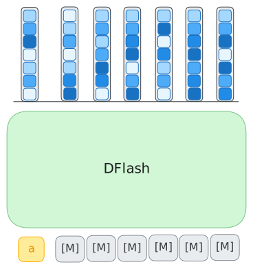
DFlash was an attempt to break the bottleneck with a diffusion model. It starts with a block of mask tokens and predicts every position at once. An eight-token draft takes one model invocation just as a one-token draft does. The wider block is not literally free, but it avoids the eight dependent forward passes required by an autoregressive drafter.

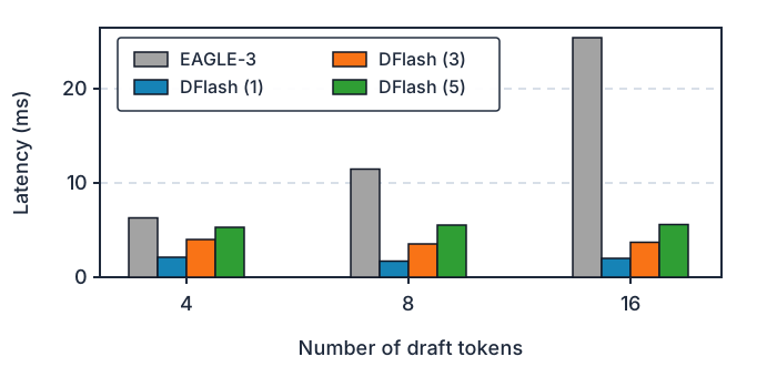
Bar chart showing EAGLE-3 draft latency increasing with the number of draft tokens while DFlash latency remains nearly constant — EAGLE-3's autoregressive drafting latency grows with the number of proposed tokens. DFlash generates the block in parallel, so its latency stays nearly constant—even with a deeper five-layer drafter. Adapted from the DFlash paper.

This makes diffusion a particularly natural fit for speculation. DFlash does not need to be a good standalone language model: the large autoregressive model will reject its mistakes. It only needs to produce plausible blocks quickly and be right often enough to save work overall.

The problem with parallel generation

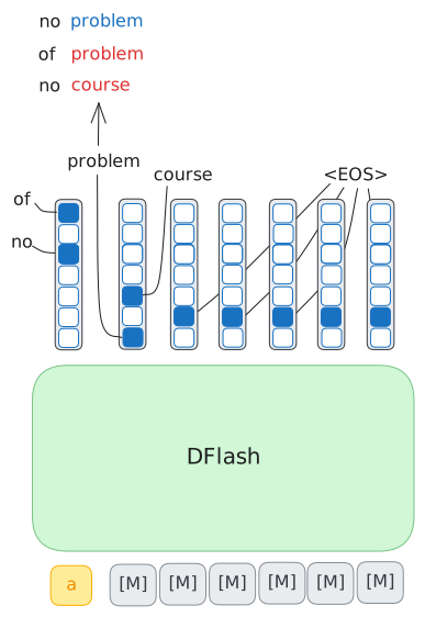
Parallel sampling mixing the phrases no problem and of course into inconsistent completions — Each position can be plausible on its own while the completed phrase is nonsense. In the above image we show a very simplified vocabulary with only 7 tokens. DFlash successfully predicts the next tokens but cannot model the dependencies between the tokens at sampling time.

The trouble is that a sequence is not a bag of independently plausible tokens.

Suppose the next two tokens could form either “no problem” or “of course”. A well-trained parallel model might put high probability on both “no” and “of” in the first position, and on both “problem” and “course” in the second. If the two positions are sampled independently, there are four possible results:

no problem
of course
no course
of problem

The first two are coherent. The other two splice together halves of different continuations. Nothing is obviously wrong with either token considered in isolation; the error is in the relationship between them.

An autoregressive model does not have this particular problem. Its first sampling decision breaks the symmetry. Once it samples “of”, that token becomes part of the input for the next step and “course” becomes much more likely than “problem”. Once it samples “no”, the reverse is true.

A diffusion model can recover this consistency by denoising repeatedly, feeding accepted choices back into later passes. That costs forward passes, however, which is exactly what a fast speculative drafter is trying to avoid. DSpark takes a cheaper route: keep the expensive part parallel and make only the sampling step autoregressive.

A parallel backbone with autoregressive sampling

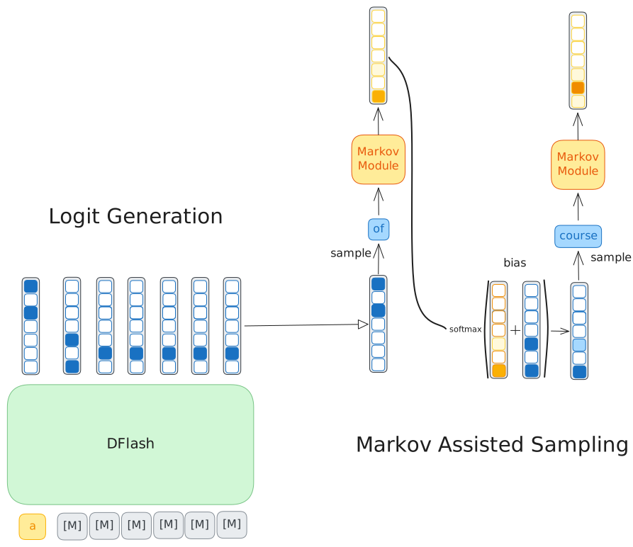
DFlash logits combined with a Markov transition bias before each token is sampled — DFlash predicts the whole block in parallel. A small Markov module then biases each position using the previously sampled token. This Markov module is effectively a bi-gram language model that models in the training corpus common next tokens that follow a given token.

DSpark calls this Semi-Autoregressive Generation. DFlash still produces logits for every position in the draft with one parallel forward pass. Before sampling a position, DSpark adds a second set of logits produced from the token sampled at the previous position.

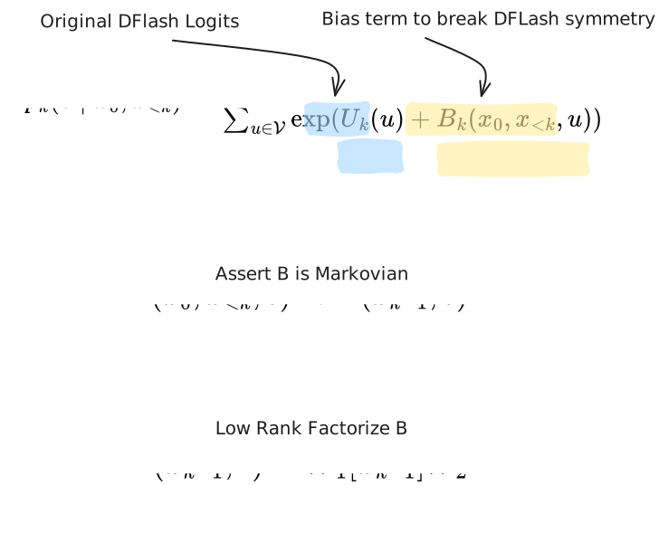
DSpark adds a general bias term to logits. — DSpark adds a bias term to the DFlash logits. In principle this bias term could condition on the entire sequence up to that point, much like a transformer would. The bias is restricted to be Markovian and low-rank to make it efficient.

The process for generating this bias logit is Markovian which means that this small module carries no state beyond its latest input. It does not know the prompt, the DFlash hidden states, or the full sequence of choices made so far. It only answers a narrow question: given the token I just sampled, which tokens tend to come next?

So if the sampler chooses “of” at the first position, the Markov module gives “course” a larger positive bias than “problem” at the second. This is because in your training corpus “no problem” is almost certainly more common than “no course”. If it chooses “no”, it favours “problem”. DFlash still supplies almost all of the linguistic knowledge. The Markov logits merely couple adjacent sampling decisions strongly enough to break the symmetry.

This is an autoregressive process, but a very cheap one. The large neural network has already run across the entire block. The serial loop contains only a lookup, a small projection, an addition, and sampling. That is a much better critical path than running a transformer once per draft token.

How the Markov sampler works

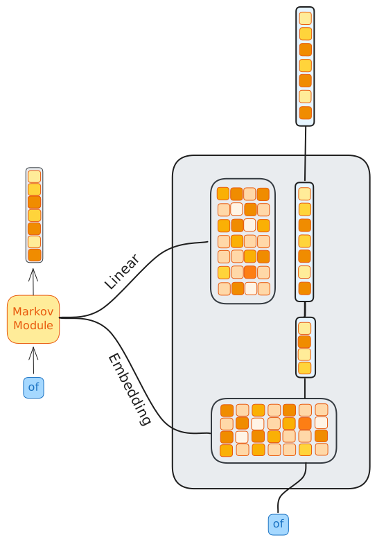
A token embedding lookup followed by a matrix projection into vocabulary logits — *The sampler is a low-rank factorisation of a vocabulary-to-vocabulary transition table.*

The Markov module has two learned matrices. The first is an embedding table: the previous token selects one vector. The second projects that vector back into vocabulary-sized logits.

If the vocabulary has size $V$ and the embedding has width $r$ , the module is equivalent to factoring a $V \times V$ token-transition matrix into a $V \times r$ lookup table and an $r \times V$ projection. A full transition matrix would directly store a score for every possible pair of adjacent tokens. The factorised version compresses that table through a much smaller intermediate dimension.

In language-model terminology this is closest to a bigram model: the distribution of the next token is conditioned on one previous token. It has none of the context sensitivity of DFlash, but it does not need it. Its job is to express simple local preferences that DFlash’s independent sampling cannot enforce.

The matrices are trained alongside DFlash. You could instead estimate a transition table from the training corpus and factorise it afterwards. Since DFlash is already being trained, learning the two matrices jointly is simpler and lets them specialise in correcting the backbone’s errors rather than merely reproducing corpus counts.

There is also a hardware tradeoff hidden in the factorisation. If memory were abundant but projection compute or repeated weight reads were expensive, the two matrices could be multiplied together ahead of time. Sampling would then become one lookup in a dense $V \times V$ table. That table becomes enormous for a modern vocabulary, which is why the low-rank form is the sensible default.

Training DSpark

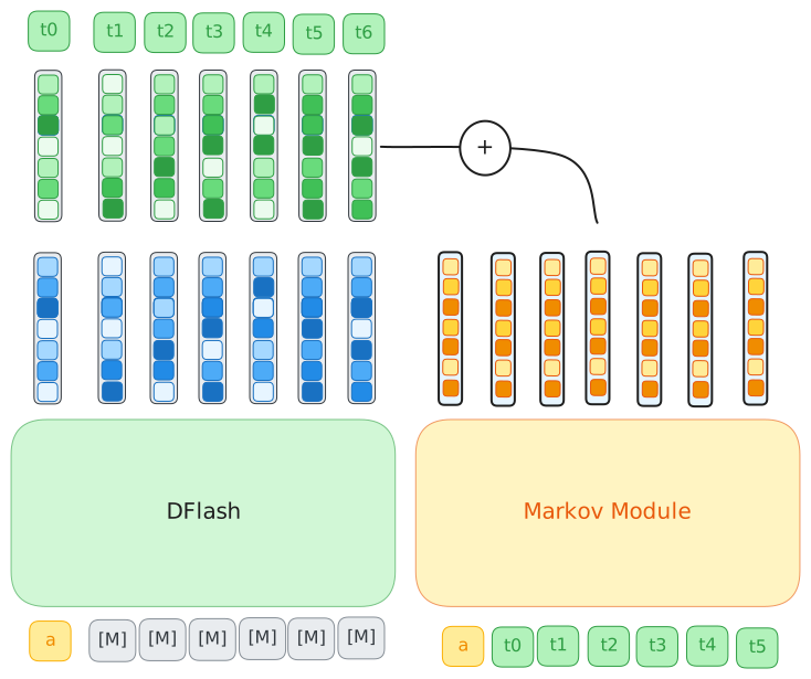
Parallel training of the DFlash backbone and Markov module using ground-truth previous tokens — *Teacher forcing keeps training parallel: every Markov input comes from the ground-truth sequence.*

At training time, DFlash receives the masked draft block and predicts logits for all of its positions. In parallel, the Markov module receives the ground-truth token immediately before each position and produces its bias logits. The two sets of logits are added, normalised with a softmax, and compared with the ground-truth continuation.

Using the ground-truth previous tokens is the important trick. At inference time the Markov sampler must run from left to right because each input is the result of the preceding sample. During training all of those inputs are already known. The Markov calculations can therefore run across the sequence in parallel, with no need to backpropagate through a chain of sampled decisions.

DSpark uses three losses to train the combined drafter:

A standard cross-entropy loss on the ground-truth tokens.
An L1 loss between the full teacher and student logit distributions, which provides the usual knowledge-distillation signal.
A confidence loss that trains the drafter to predict whether its tokens will be accepted by the target model.

That last prediction is useful at serving time. A speculator has to decide how far ahead it should draft. When it expects a continuation to be easy, it can propose a longer block; when its confidence drops, it can stop before spending work on tokens that are likely to be rejected. Draft models are often good judges of where their own guesses become unreliable, so confidence is part of the decoding policy rather than just a diagnostic.

What comes after Markov sampling?

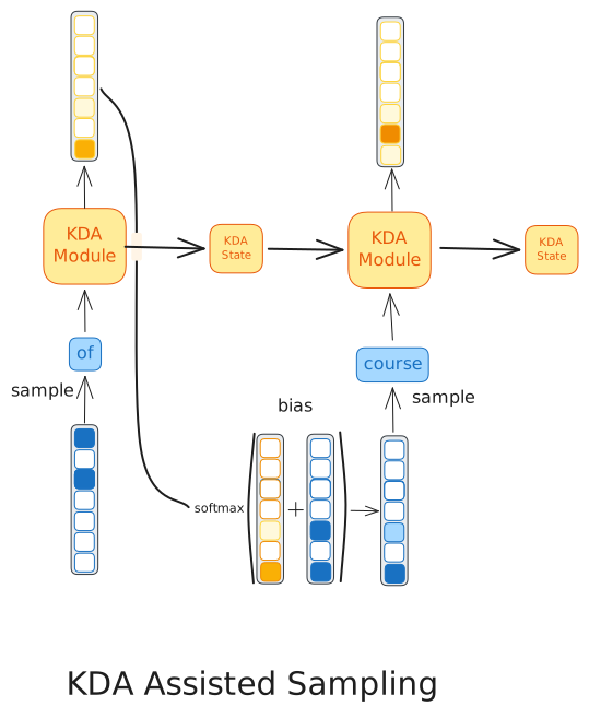
A proposed Kimi Delta Attention sampler carrying recurrent state between sampling steps — *A recurrent sampler could remember more than the previous token while leaving the DFlash backbone parallel.*

The Markov module is the smallest useful autoregressive addition to DFlash. It remembers one token and discards everything else. That simplicity keeps it fast, but it also suggests several obvious extensions.

The first is to give it a little more discrete context. DeepSeek has already experimented with n-gram embeddings: separate learned vectors for individual tokens and for token pairs found in the training corpus. A DSpark sampler could condition on the last two or three tokens rather than only the last one. The difficulty is memory. The number of possible n-grams grows rapidly, and even the subset observed in a corpus can make for a very large embedding table. Another low-rank factorisation may make this practical.

The other route is a recurrent neural module. The DSpark work experiments with a simple RNN, but there is no reason to stop there. Recent language models have made effective use of recurrent layers such as Mamba, Gated DeltaNet, and Kimi Delta Attention. These modules have cheap recurrent steps and can carry a compact state summarising earlier decisions.

The final diagram sketches a KDA-assisted sampler. Instead of mapping only the last token to a bias, it passes a state from one sampling step to the next. That state gives the sampler a short record of the path it has taken through the draft. DFlash would still do the expensive contextual reasoning in parallel; KDA would supply enough serial memory to keep the sampled continuation on one coherent path.

There is a continuum here. At one end is independent sampling: maximally parallel and prone to mixing incompatible continuations. At the other is a full autoregressive transformer: coherent, expressive, and expensive. DSpark picks a useful point close to the parallel end. Its result is not that autoregression was unnecessary. It is that only a very small amount of it was needed.