NOTE: while writing this post I came across a similar set of ideas posted on LessWrong. Check that out for an alternative presentation of a similar idea!

Attention variants have a way of looking more intimidating than they really are.

The equations are not impossible, but they are fiddly. A lot of the work is just keeping track of which dimensions have been split, shared, compressed, or reabsorbed into some neighboring projection matrix.

Tensor networks hold a special place in my heart. I did a PhD centered around tensor networks, and we started Doubleword by looking at ways we could compress computer vision models with tensor networks. They don’t get used much these days when it comes to performance engineering in LLMs but I still tend to approach linear algebra equations through a tensor network lens.

Tensor network notation is useful here because it turns those index games into pictures. Instead of repeatedly asking “which matrix can I multiply into which other matrix?”, you can look for adjacent nodes in the graph and contract them.

In this post I want to build up a tensor-network view of attention, starting from a generic bilinear attention operator and ending at DeepSeek’s MLA. The point is not that tensor networks make the kernels faster. The point is that they make the structure visible, and once the structure is visible it becomes much easier to see which existing fast kernel an attention variant can be mapped onto.

Tensor Networks in One Page

Tensor networks are a visual language for tensor operations.

The rules are simple:

• A tensor is a node.
• Each dimension of the tensor is a line coming out of that node.
• An open line is an output dimension.
• A connected line is a summed-over dimension.

So a vector is a node with one line, a matrix is a node with two lines, and a rank-3 tensor is a node with three lines. Matrix-vector multiplication is just a matrix node connected to a vector node along one shared index. The result has one open line, so it is a vector.

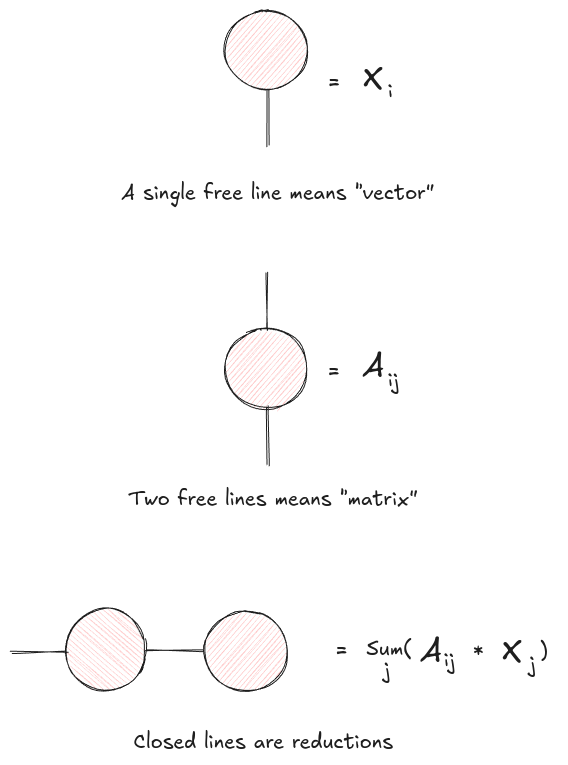
Figure 1: Tensor network notation replaces index summations with connected lines. A contraction over a shared index is drawn by joining the corresponding legs.

This is the whole game. If two nodes are connected, that index is summed over. If they are not connected, that index remains visible in the output.

For attention, the useful part is that tensor-network diagrams make factorization explicit. If a large tensor can be written as the product of two smaller tensors, the diagram gets an extra internal line. That internal line is the compressed dimension. In ordinary linear algebra you would call this a low-rank factorization.

Start With Bilinear Multi-Head Attention

Let $X \in \mathbb{R}^{L \times H}$ be the hidden states for a sequence of length $L$ and hidden size $H$.

The most general attention-like object we will look at is a set of bilinear forms:

$$A_n = X W_n X^T$$

where each $W_n \in \mathbb{R}^{H \times H}$ is a learned bilinear operator for head $n$.

This already has the essential attention shape. Every token interacts with every other token, because the result $A_n$ has two sequence dimensions: one for the query token and one for the key token. After that we apply a nonlinearity, usually softmax, and use the resulting attention matrix to mix token representations. We then concatenate the results of the different heads together, and multiply this vector by a matrix.

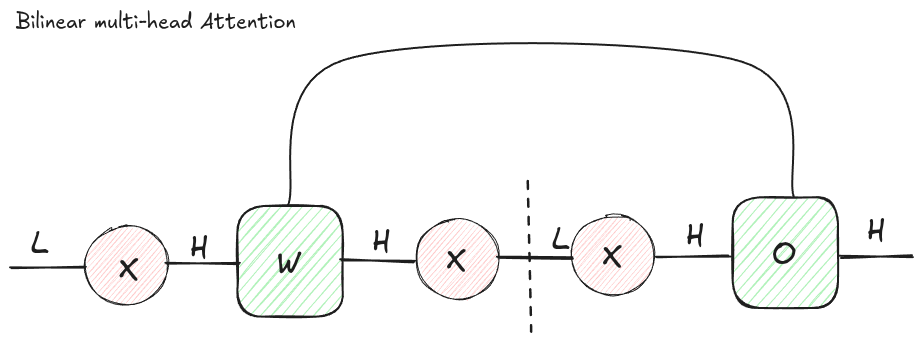Figure 2: A generic bilinear attention layer. Each head owns a full bilinear operator $W_n$, producing one attention matrix per head.

There is one important wrinkle in the diagram: the dotted line around the softmax.

In a pure tensor network, you can freely contract neighboring linear operators in almost any order. Softmax ruins that freedom. Once you compute the attention logits, you must apply the nonlinearity before multiplying by values. That means you cannot just contract the value projection into the bilinear operator and pretend the whole thing is one big linear map.

This is one of the places where the diagram earns its keep. It tells you which rearrangements are legal linear algebra and which ones cross the nonlinear boundary.

Standard Multi-Head Attention

Standard multi-head attention appears when we factor each bilinear operator:

$$W_n = W_{Q,n} W_{K,n}^T$$

with an internal dimension $d$.

Then:

$$Q_n = X W_{Q,n}, \quad K_n = X W_{K,n}$$

and the logits are:

$$A_n = Q_n K_n^T$$

That is the familiar attention score computation.

We can do the same thing to the output side. Instead of treating the final output map as one large opaque tensor, split it into a per-head value projection and a shared output projection:

$$V_n = X W_{V,n}$$

Then concatenate the per-head attention outputs and apply $W_O$.

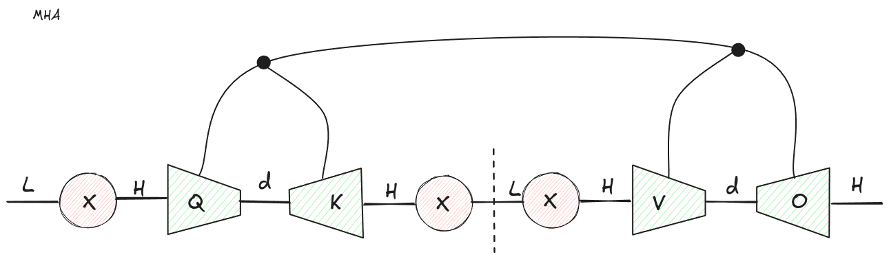Figure 3: Standard MHA falls out by factorizing each bilinear operator into query and key projections, and factorizing the output side into value and output projections.

This is the early transformer implementation written as a tensor network.

The KV cache story also becomes visible. During decoding, the current token supplies the new query, but every previous token contributes keys and values. So we cache $K$ and $V$ rather than caching $X$ and recomputing projections every step.

MHA reduces each key and value vector from hidden size $H$ to head size $d$, but it stores one key and one value per head. Since models are usually configured with $N d = H$, the total KV width is still roughly:

$$2Nd = 2H$$

per token per layer.

That is the quantity all the later variants are trying to attack.

Multi-Query Attention as KV Cache Compression

Multi-query attention (MQA) makes a simple trade: keep multiple query heads, but share keys and values across those heads.

From bilinear attention you can group the query index and head index together, and perform an SVD with this joint index and the key index.

Instead of each head having its own key projection $W_{K,n}$ and value projection $W_{V,n}$, all heads use the same $W_K$ and $W_V$. The query side still has a head dimension, so the model can ask many different questions of the same cached memory.

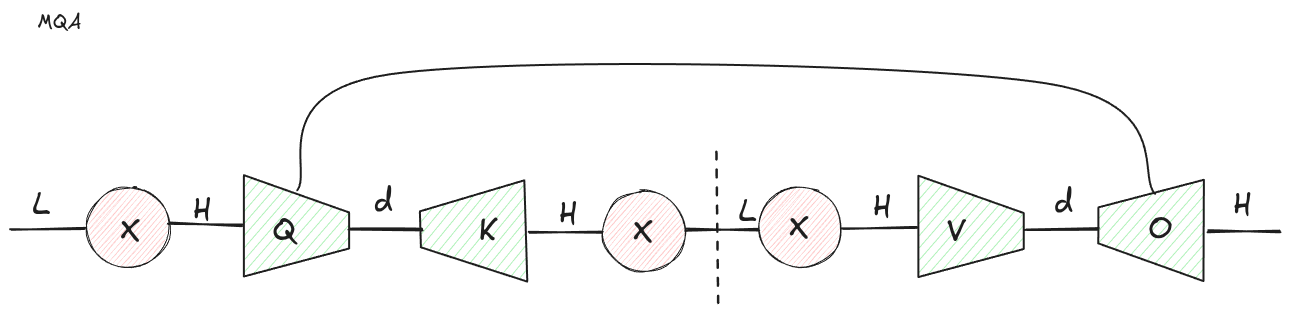Figure 4: MQA shares the key and value projections across heads. The head dimension remains on the query side, but disappears from the cached K and V tensors.

In tensor-network language, we have changed where the head index lives.

For MHA, the head index is present on the cached K and V tensors. For MQA, the head index is pushed into the query-side projection and the final output mixing. The cached tensors are now:

$$K \in \mathbb{R}^{L \times d}, \quad V \in \mathbb{R}^{L \times d}$$

instead of:

$$K,V \in \mathbb{R}^{L \times N \times d}$$

That is a factor of $N$ reduction in KV cache size.

This reduction is not free. MQA is less expressive than MHA because every query head attends to the same key and value representation. But for decoding, KV cache bandwidth is often the bottleneck, and saving a factor of $N$ is a very large hammer.

Grouped-query attention sits between these two extremes: several query heads share each KV head. In the diagram you would keep a smaller KV-head index instead of deleting it entirely.

Talking-Heads Attention

Once the bilinear picture is in place, more exotic variants become easier to reason about.

One example is Talking-Heads Attention, introduced by Shazeer, Lan, Cheng, Ding, and Hou in 2020. The paper adds learned linear projections across the head dimension immediately before and after softmax.

In normal MHA, each head computes its own attention matrix and then values are mixed independently per head until the final output projection. Talking-heads attention lets the attention heads communicate while they are still attention matrices.

That means the model can form logits in one set of heads, mix those logits across heads, apply softmax, and optionally mix the resulting probabilities across heads again.

FlashAttention-style kernels avoid materializing the full $L \times L$ attention matrix. The attention probabilities exist only transiently, tiled through SRAM inside the kernel. A projection across the head dimension at the attention-matrix stage is therefore awkward: the thing you want to mix is deliberately never written out as a convenient dense tensor.

That is probably one reason talking-heads attention has not become a standard LLM serving primitive, despite being a clean architectural idea.

The tensor network view shows two ways to get talking-heads-like structure.

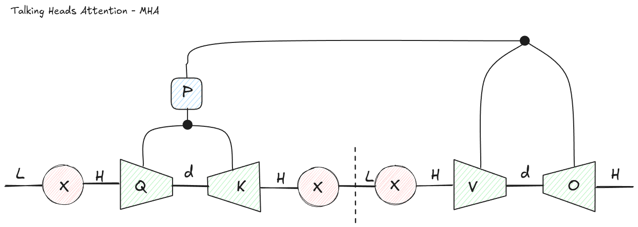Figure 5: In an MHA-like factorization, the projection across heads remains visible as a separate tensor acting on the head dimension.

For an MHA-style version, start from the bilinear operator with a head dimension. Factor it so that one piece is a projection across heads, and the remaining pieces look like ordinary per-head query and key projections. The head-mixing matrix cannot generally be ignored because it acts across the separate attention matrices.

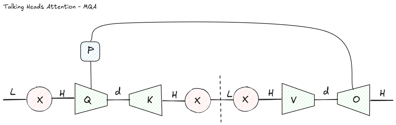Figure 6: In an MQA-like factorization, the head-mixing projection can be absorbed back into the query projection.

For an MQA-style version, something funny happens. Since keys are shared, the head-specific structure is mostly on the query side. A linear projection across heads can be reabsorbed into the query projection itself. In other words, the talking-heads MQA diagram collapses back into ordinary MQA.

That does not prove the variant is useless in every possible implementation. But it does show that, under this factorization, the extra projection is not buying you a new kind of expressivity. It is just a different parameterization of the same computation.

This is exactly the sort of thing tensor diagrams are good for. You can often see when a proposed architectural component is genuinely new, and when it is just a matrix waiting to be multiplied into its neighbor.

Multi-Head Latent Attention

DeepSeek introduced Multi-head Latent Attention in DeepSeek-V2, published in 2024. The headline motivation was inference efficiency: compress the KV cache into a latent vector while retaining more expressivity than plain MQA.

Ignoring positional embeddings for a moment, the core MLA idea is to insert a shared latent bottleneck before keys and values:

$$c^{KV} = X S_{KV}$$

Then keys and values are produced from this latent:

$$K_n = c^{KV} W_{K,n}, \quad V_n = c^{KV} W_{V,n}$$

The query side can also be factorized through its own latent:

$$c^Q = X S_Q, \quad Q_n = c^Q W_{Q,n}$$

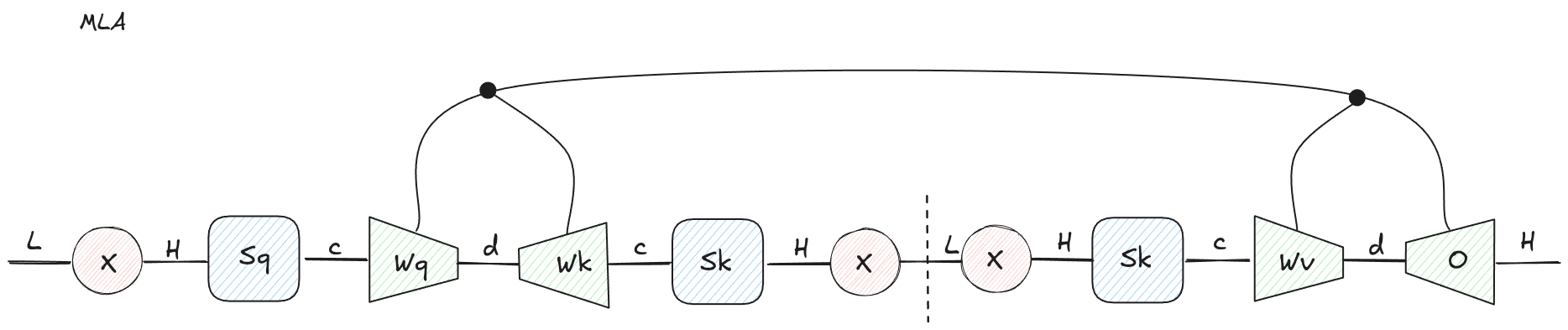Figure 7: MLA inserts a latent bottleneck. Instead of caching per-head keys and values, the model can cache the shared latent $c^{KV}$.

This looks like a small change, but it matters a lot for serving.

In MHA, the cache stores per-head keys and values:

$$2Nd$$

numbers per token per layer.

In MQA, the cache stores one shared key and one shared value:

$$2d$$

numbers per token per layer.

In MLA, the cache stores one latent vector:

$$c$$

numbers per token per layer, where $d < c < Nd$ in the usual regime.

So MLA is less aggressively compressed than MQA, but more expressive. The latent can contain more information than a single MQA key/value pair, while still being much smaller than the full MHA KV cache. It is also only cached once, not once for keys and once for values.

The DeepSeek-V2 paper reports that MLA reduces KV cache size substantially, and that this is a major contributor to higher maximum generation throughput. That matches the basic serving intuition: decoding often spends more time moving KV cache than doing math, so shrinking the cache changes the roofline.

The real trick is that MLA has two useful execution views.

MLA as MHA

For training and prefill, you usually care about large dense matrix multiplications over many tokens. In that regime, it is often convenient to materialize the ordinary per-head Q, K, and V tensors and use an MHA-style implementation.

The tensor network tells you how to do that: contract adjacent linear maps before the attention operation.

For example, the query path:

$$X \rightarrow S_Q \rightarrow W_Q$$

can be collapsed into a single effective query projection:

$$\widetilde{W}_Q = S_Q W_Q$$

Likewise, the KV latent path can be collapsed into effective key and value projections:

$$\widetilde{W}_K = S_{KV} W_K, \quad \widetilde{W}_V = S_{KV} W_V$$

Now the layer looks like normal MHA.

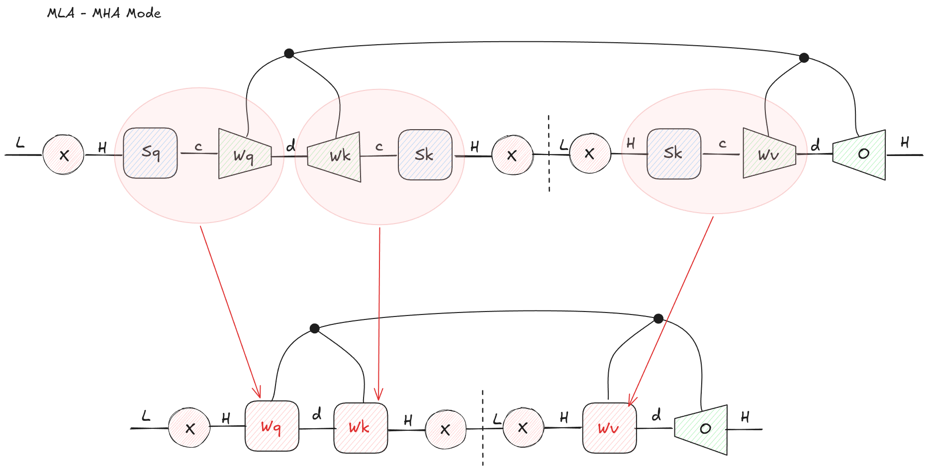Figure 8: MLA can be contracted into an MHA-shaped computation by combining the down-projection and up-projection matrices on each path.

This mode does not preserve the KV-cache advantage, because it expands the latent back into per-head K and V. But during prefill, that may be the right trade. Prefill is a dense parallel workload, and using an existing optimized MHA path is attractive.

DeepSeek describe using this kind of mode for training and prefill, where compute efficiency matters more than minimizing the per-token decode cache.

MLA as MQA

During decoding, the bottleneck changes. The query length is usually one token, and the expensive part is repeatedly loading the cached history. This is where MLA’s latent cache matters.

The tensor network gives a second contraction pattern: instead of expanding cached latents into K and V, absorb the key and value up-projections into the query and output-side projections.

For the attention score:

$$\begin{aligned} Q_n K_n^T &= (c^Q W_{Q,n})(c^{KV} W_{K,n})^T \end{aligned}$$

Rearrange the linear maps:

$$\begin{aligned} Q_n K_n^T &= c^Q (W_{Q,n} W_{K,n}^T) (c^{KV})^T \end{aligned}$$

So the cached object can remain $c^{KV}$. You transform the query side so that it compares directly against the latent cache.

The same idea applies to values and the output projection. Instead of first expanding:

$$V_n = c^{KV} W_{V,n}$$

and then applying $W_O$, contract $W_V$ and $W_O$ into the output side. The attention kernel can read the latent cache and produce an output that is then mapped back to hidden size.

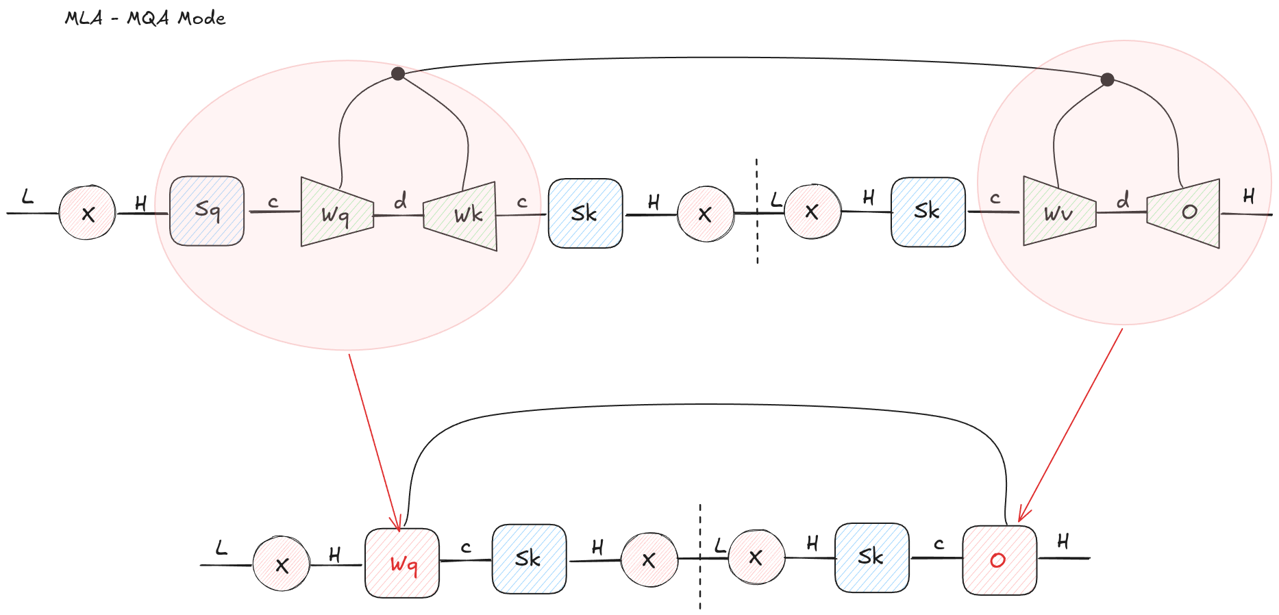Figure 9: MLA can also be contracted into an MQA-shaped decode path. The cached tensor remains the compressed latent rather than expanded per-head K and V.

This is why MLA has an MQA-like serving mode. The kernel sees a shared cached representation, so it has the memory behavior you want for decoding. But the projections around that shared cache are richer than plain MQA.

Said differently: MQA says “all heads share this small KV representation.” MLA says “all heads share this larger latent representation, and each head can read from it through learned maps.”

That is a much nicer point in the design space.

What the Diagram Makes Obvious

A few patterns become obvious:

• MHA is a low-rank factorization of a per-head bilinear attention operator.
• MQA is a low-rank factorization of the entire bilinear attention operator from the space of input vectors and heads to the output vector.
• Talking-heads attention adds a real head-mixing operation in the MHA case, but an MQA-like version can collapse back into the query projection.
• MLA is a shared latent bottleneck for keys and values, with two different contraction orders: expand to MHA for prefill, or preserve the latent cache for MQA-like decoding.

Tensor-network notation gives you a compact way to reason about attention variants that is more intuitive than just working through the equations.

Conclusion

Most attention variants are rearrangements of the same few ingredients: bilinear token-token interaction, low-rank factorization, head sharing, latent compression, and output mixing.

The hard part is not writing down the equations. The hard part is seeing which dimensions are really necessary at runtime.

That is why tensor networks are a useful tool for LLM systems work. They make it visually obvious when two matrices can be fused, when a projection is blocked by softmax, and when a cache can be stored in a smaller latent space without changing the computation you need during decoding.

The next time a new attention mechanism shows up, it is worth drawing the tensor network before reaching for a custom kernel. There is a decent chance the new thing is one contraction away from a kernel you already have.