Pricing a language model starts with a benchmark that looks like the traffic you intend to serve. Send requests in parallel, count the input and output tokens the server actually processes, and measure how long the deployment takes to process them. Once you know the amount of useful work a server does per hour, you can put a cost under it.

The awkward part is deciding which requests to send. A deployment serving 200 short chat completions does not have the same economics as one serving two 100,000-token prompts. An agent that can reuse almost all of its growing history through prefix caching does not cost the same as an agent that repeatedly prefills that history from scratch.

BatchBench is a small library for constructing these workloads, sending them to an OpenAI-compatible API in parallel, and recording elapsed time, latency, failures, and server-reported input and output token counts. This post starts by walking through its design, then uses the measurements it produces to price a model.

The shortest useful benchmark

Suppose the product you want to price usually receives 8,192 input tokens and produces 1,024 output tokens. A fixed-shape run against a local SGLang server looks like this:

uv pip install batchbench

batchbench \
  --model Qwen/Qwen3-8B \
  --host http://localhost:8000 \
  --users 64 \
  --requests-per-user 4 \
  --input-tokens 8192 \
  --output-tokens 1024 \
  --sglang \
  --seed 7 \
  --results-csv 8k-in-1k-out.csv

--users 64 creates 64 independent workers. Each worker sends four requests sequentially, while the workers run concurrently. This distinction is useful: a user represents one in-flight sequence, rather than a one-off burst of 256 requests with no control over concurrency.

BatchBench generates 256 prompts with the model’s tokenizer, asks the server for a fixed-size completion, and sends each request to /v1/chat/completions. The response must contain the usual OpenAI usage.prompt_tokens and usage.completion_tokens fields. Those server-reported values—not the requested lengths—are accumulated into the final report.

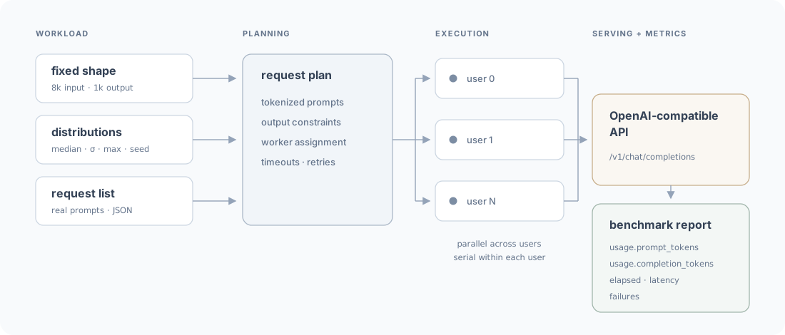
The important totals are:

total_duration
total_prompt_tokens
total_completion_tokens
prompt_tokens_per_second
completion_tokens_per_second
requests_per_second
latency_p50 / latency_p90 / latency_p99

Throughput is aggregate throughput across the deployment. If 200 requests each decode at 20 tok/s, the server is producing 4,000 tok/s. Per-request speed tells you what a customer experiences; aggregate speed tells you how much hardware time each token consumes.

How BatchBench constructs prompts

The library can take a list of supplied request bodies, but it can also synthesize prompts with a chosen token length. The generator first chooses a length for every request. It then samples synthetic token IDs that the selected tokenizer can decode, turns them into text, and places the text in an OpenAI chat request.

The central part of generator.rs is approximately:

let sequence_lengths = sample_lengths(&options, &mut rng)?;

for (line_idx, seq_len) in sequence_lengths.into_iter().enumerate() {
    let ids: Vec<u32> = (0..seq_len)
        .map(|_| rng.gen_range(1..=10_000))
        .collect();
    let prompt = tokenizer.decode(&ids, true)?;

    requests.push(RequestEntry {
        body: json!({
            "model": model,
            "messages": [{"role": "user", "content": prompt}],
        }),
        line_idx,
        input_tokens: seq_len,
    });
}

Generating from tokens rather than repeating a word gives the server a realistically sized prompt without requiring a dataset for every point in a sweep. Decoding and re-tokenizing can change the exact count, which is another reason to use the API’s usage object as the final measurement.

BatchBench can also make a fraction of the prompt common across requests with --input-prefix-overlap. This is useful for workloads with a shared system prompt. It is different from the agent cache benchmark later in the post: prefix overlap creates a common prefix across independent users, while agent mode grows and resends one conversation per agent.

The concurrency model

The Rust runner.rs uses Tokio’s JoinSet to launch one task per simulated user. Boiled down to its scheduling structure, it looks like this:

let mut workers = JoinSet::new();

for user_id in 0..config.user_count {
    let client = client.clone();
    let config = Arc::clone(&config);
    let events = event_tx.clone();

    workers.spawn(async move {
        run_user(user_id, client, config, events).await
    });
}

while let Some(worker) = workers.join_next().await {
    worker??;
}

Inside run_user, requests are sent one after another. Across users they overlap. Successful responses send a small event containing latency, prompt tokens, and completion tokens to a metrics task. The relevant part of the response handling boils down to:

let usage = payload
    .get("usage")
    .context("response missing usage field")?;

let prompt_tokens = usage["prompt_tokens"]
    .as_u64()
    .context("prompt_tokens is not an integer")?;
let completion_tokens = usage["completion_tokens"]
    .as_u64()
    .unwrap_or(0);

events.send(WorkerEvent::Success {
    prompt_tokens,
    completion_tokens,
    latency: started.elapsed(),
})?;

The runner therefore has three fairly clean pieces: request generation, concurrent workers, and a metrics aggregator. You can change the workload shape without changing the HTTP runner, or add report outputs without changing how requests are constructed.

Fixed requests are useful, but distributions are more honest

The 8k-in, 1k-out run gives a clean point on the performance surface. It is good for comparisons and regression tests. Most production request streams do not sit at one point.

Language-model request lengths are positive, right-skewed, and often have a long tail. A log-normal distribution is a useful first model of that shape. It is not a law of nature, but it is substantially more representative than pretending every request is the average request.

BatchBench can independently sample the input and output length for every request:

batchbench \
  --model Qwen/Qwen3-8B \
  --host http://localhost:8000 \
  --users 64 \
  --requests-per-user 20 \
  --input-lognorm-median 8192 \
  --input-lognorm-sigma 0.8 \
  --input-lognorm-max 32768 \
  --output-lognorm-median 1024 \
  --output-lognorm-sigma 0.6 \
  --output-lognorm-max 8192 \
  --sglang \
  --seed 7

The median is usually easier to reason about than the log-space parameter $\mu$, so the CLI accepts either. For a log-normal distribution,

$$\operatorname{median}(X)=e^\mu, \qquad \operatorname{mean}(X)=e^{\mu+\sigma^2/2}.$$

As $\sigma$ grows, the mean moves further above the median. The max arguments truncate extreme samples so a benchmark cannot accidentally produce a prompt larger than the model’s context window. A seed makes the samples reproducible.

Figure 2 puts the two workload models on linear token axes. Set the fixed input and output lengths on the left, or change each log-normal median and $\sigma$ on the right to see how the sampled workload moves, spreads, and develops a longer right tail.

Workload shape explorer

Fixed points and sampled distributions

Drag a slider or enter a value

Input sequence length (ISL)Output sequence length (OSL)Each series is normalized independently.

Fixed

Two point masses

Every request has the same length.

Input length (ISL)tokOutput length (OSL)tok

Log-normal

Sampled request lengths

Median moves the curve; σ changes its width.

Input mediantokInput sigmaσ

Output mediantokOutput sigmaσ

For a serious pricing exercise I would run both:

1. A grid of fixed input length, output length, and concurrency. This maps the deployment’s performance surface and makes regressions interpretable.
2. A sampled workload fitted to production traces. This tells you where on that surface the product actually spends its time.

An average input length and an average output length are not enough. A run containing one 32k-token request and thirty-one 1k-token requests can schedule differently from a run containing thirty-two 2k-token requests, even though both contain the same number of input tokens.

Why different request shapes have different prices

There is no single physical cost for an input token or an output token. There is a cost for running a particular mixture of requests on particular hardware under a latency target.

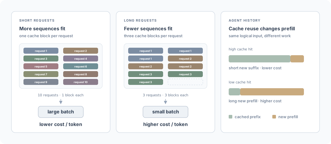
Short requests leave more KV-cache capacity available, so the scheduler can keep a larger batch of sequences in flight. Larger batches reuse each weight load across more tokens and generally make the GPU cheaper per token. Long prompts and long generations occupy more KV cache, reduce the batch the server can sustain, and can move the deployment to a more expensive operating point.

The same effect appears across the prefill and decode phases:

• Prefill reads the prompt and builds the KV cache. It processes many input tokens in parallel and is often compute-bound.
• Decode generates the answer one token at a time. It repeatedly loads model weights and is often memory-bandwidth-bound, so it depends heavily on batching many sequences.

This is why output tokens usually cost more than input tokens, and why the ratio is workload-dependent. A batch-of-one decode benchmark measures latency, not the economics of a busy serving system.

Agent mode: benchmark the conversation, not just the turn

Agent traffic breaks a stateless benchmark. An agent sends a prompt, receives a tool call, waits for the tool, appends the result, and sends the whole conversation again. On the third request, most of the input is identical to the second request; only the latest model response and tool result are new.

If the inference server retains the prefix cache, it can reuse the KV state for that shared history. A high cache-hit workload has a short incremental prefill and is cheap. A low cache-hit workload repeatedly computes a long prefill and is expensive. Counting only the logical number of input tokens does not reveal the difference.

BatchBench’s batchbench-agent entrypoint models this directly:

batchbench-agent \
  --model Qwen/Qwen3-8B \
  --host http://localhost:8000 \
  --agents 32 \
  --input-tokens 4096 \
  --output-tokens 256 \
  --environment-tokens 512 \
  --tool-invocations 8 \
  --tool-call-latency-ms 250 \
  --sglang \
  --seed 7

This launches 32 independent agents in parallel. Within one agent, turns stay sequential because the next request depends on the previous model response and tool result. The 250ms sleep represents work happening in the environment; while one agent waits, other agents can continue to use the server.

The same values can be sampled. Agent mode accepts log-normal specifications for the initial prompt, model response, environment response, number of tool invocations, and tool-call latency. This produces different conversation lengths and natural gaps between requests, rather than 32 identical metronomes.

The public Rust API in agent.rs exposes the same design:

use batchbench_rs::{
    run_agent_benchmark, AgentLoopConfig, SampleSpec,
};

let config = AgentLoopConfig::try_new(
    "http://localhost:8000/v1/chat/completions",
    None,
    "Qwen/Qwen3-8B",
    32,                                        // parallel agents
    SampleSpec::fixed(4_096)?,                 // initial prompt
    SampleSpec::log_normal_from_median(256.0, 0.5, Some(2_048))?,
    SampleSpec::log_normal_from_median(512.0, 0.7, Some(4_096))?,
    SampleSpec::fixed(8)?,                     // turns per agent
)?
.with_tool_call_latency_ms(
    SampleSpec::log_normal_from_median(250.0, 0.4, Some(2_000))?
)?
.with_seed(7)
.with_sglang(true);

let report = run_agent_benchmark(config).await?;

Before sending anything, BatchBench samples a complete AgentPlan for every agent. Separate seeded random-number streams are used for input length, output length, environment length, turn count, text, and tool latency, so changing one distribution does not reshuffle all of the others.

Every request advertises one synthetic environment function and forces the model to call it. BatchBench retains the assistant’s tool-call message, generates an environment response of the sampled length with the same tokenizer, and sets parallel_tool_calls to false so each turn has one serial environment step. If a compatible server returns an assistant message without a tool call, BatchBench adds a synthetic one so the conversation can continue.

The initial message is just a generated user prompt:

let mut messages = vec![json!({
    "role": "user",
    "content": plan.initial_prompt,
})];

After each successful response, BatchBench keeps the returned assistant message, sleeps for the sampled tool time, and appends a synthetic tool response:

messages.push(assistant_message);
messages.push(json!({
    "role": "tool",
    "tool_call_id": tool_call_id,
    "content": turn.environment_content,
}));

// The next request resends the complete, growing message history.
let body = build_request_body(&config, &messages, turn.output_tokens);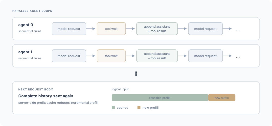

The agent report includes total server-reported input and output tokens, tool time, end-to-end duration, throughput, latency percentiles, and estimated_cached_input_tokens. The cache estimate is the previous prompt length capped by the current prompt length, which is the optimistic reusable prefix if the server caches perfectly. It is an estimate, not a measurement of physical cache hits: eviction, block boundaries, routing, and the server’s cache implementation can all reduce actual reuse.

That difference is exactly what makes agent mode useful. Compare runs with prefix caching enabled and disabled, or compare servers under the same plan. The logical token totals remain similar while elapsed time and server-side work change.

Turn a BatchBench run into a price

Start from the pricing equation. If a BatchBench run serves $I$ input tokens and $O$ output tokens, then a pair of per-token prices $p_\text{input}$ and $p_\text{output}$ reaches the target when

$$\boxed{ C_\text{run}M = p_\text{input}I + p_\text{output}O }$$

Here $C_\text{run}$ is the hardware cost of the benchmark and $M$ is the margin multiplier. $M=1$ recovers the measured hardware cost; $M=1.25$ targets 25% more revenue than that cost. This is a markup multiplier rather than the accounting definition of gross margin.

If the complete GPU server costs $C_\text{hour}$ dollars per hour and the run takes $T$ seconds, then

$$C_\text{run} = \frac{C_\text{hour}}{3{,}600}T.$$

API prices are normally quoted per million tokens, so write them as $P_\text{input}$ and $P_\text{output}$. The same equation becomes

$$\boxed{ C_\text{run}M = \frac{I}{1{,}000{,}000}P_\text{input} + \frac{O}{1{,}000{,}000}P_\text{output} }$$

This is one equation with two variables. It does not define one answer; it defines a straight line of valid input/output price pairs. Solving for input price gives

$$P_\text{input} = \frac{1{,}000{,}000C_\text{run}M}{I} - \frac{O}{I}P_\text{output}.$$

One end of the line assigns all revenue to input tokens:

$$\left( P_\text{output}, P_\text{input} \right) = \left( 0, \frac{1{,}000{,}000C_\text{run}M}{I} \right).$$

The other assigns all revenue to output tokens:

$$\left( P_\text{output}, P_\text{input} \right) = \left( \frac{1{,}000{,}000C_\text{run}M}{O}, 0 \right).$$

Every non-negative point between those intercepts earns exactly $C_\text{run}M$ on the measured workload. Prices above the line earn more than the target; prices below it do not cover the target.

Price-line explorer

One run, a line of possible prices

Hover or drag across the plot

Run timesecondsGPU server cost$/hrMargin multiplier× costInput tokens servedtokensOutput tokens servedtokens

Measured run cost$2.13

Revenue target after margin$2.67

2.10M input + 262.1k output tokens

$2.67=P_in × 2.10M+P_out × 0.26M

Choose a point on the line45% input-price contribution · 55% output-price contribution

Combine several runs into one pricing decision

A production service rarely has just one request shape. Suppose you benchmark $N$ representative workloads. Run $k$ serves $I_k$ input tokens and $O_k$ output tokens, and its cost after applying the margin multiplier is $R_k=C_kM$. Its price equation is

$$\frac{I_k}{1{,}000{,}000}P_{\text{input}} + \frac{O_k}{1{,}000{,}000}P_{\text{output}} = R_k.$$

Give each workload a likelihood $w_k$, with $\sum_k w_k=1$. These weights should describe the expected share of comparable units: requests, conversations, or fixed time windows.

There are three useful ways to turn those runs into a pricing decision. They answer slightly different questions.

1. Choose a point on each line, then average the points

For each workload, choose one valid pair $(P_{\text{input},k},P_{\text{output},k})$ on its line. You might assign a larger share of the cost to output for generation-heavy traffic and a larger share to input for long-context traffic. Then take the likelihood-weighted average:

$$\bar P_{\text{input}} = \sum_k w_kP_{\text{input},k}, \qquad \bar P_{\text{output}} = \sum_k w_kP_{\text{output},k}.$$

This produces a single, easy-to-explain price pair and lets business judgement influence the input/output split for each workload. The catch is that the result depends on all $N$ point choices. It also does not generally lie on the price line for the combined expected workload, so it can recover more or less than the target cost. Treat it as a policy heuristic and check its expected revenue afterwards.

2. Pool the weighted costs and tokens

Instead of combining prices, combine the measurements:

$$\bar I=\sum_k w_kI_k, \qquad \bar O=\sum_k w_kO_k, \qquad \bar R=\sum_k w_kR_k.$$

Then price the expected workload:

$$\boxed{ \frac{\bar I}{1{,}000{,}000}P_{\text{input}} + \frac{\bar O}{1{,}000{,}000}P_{\text{output}} = \bar R }$$

This line has a clean interpretation: every point on it recovers the target cost in expectation for the workload mixture described by the weights. It is usually the best default when you need one tariff and have a credible traffic forecast. It is still one equation with two unknowns, however, so you must choose where on the line to price.

3. Solve the workload equations together

Stack the workload equations into a matrix:

$$\underbrace{ \begin{bmatrix} I_1/10^6 & O_1/10^6 \\ I_2/10^6 & O_2/10^6 \\ \vdots & \vdots \\ I_N/10^6 & O_N/10^6 \end{bmatrix} }_{A} \underbrace{ \begin{bmatrix} P_{\text{input}} \\ P_{\text{output}} \end{bmatrix} }_{p} = \underbrace{ \begin{bmatrix} R_1 \\ R_2 \\ \vdots \\ R_N \end{bmatrix} }_{r}.$$

Two independent equations are enough for a unique solution. More than two equations have the same exact solution only when all of the measured price lines meet at one point.

Real measurements contain noise, so $N>2$ equations will usually be inconsistent. In that case, solve the likelihood-weighted least-squares problem

$$p^* = \arg\min_p \sum_k w_k(A_kp-r_k)^2 = (A^\mathsf{T}WA)^{-1}A^\mathsf{T}Wr.$$

This returns the price pair that minimises weighted squared cost-recovery error across the workloads. It does not generally lie on any individual line. The solution is unique when the workloads contain at least two genuinely different input/output ratios, so $A^\mathsf{T}WA$ is invertible. If every workload has the same ratio, the equations cannot identify separate input and output prices.

Multi-run price explorer

Four workloads, three ways to combine them

Show all methods

W1

Short chat

Balanced prompts and replies

40%

3M in + 1.5M out = $19.9

Likelihood weightChosen point$2.98 in · $7.30 out

W2

Long context

Prefill-heavy requests

25%

10M in + 0.8M out = $28.0

Likelihood weightChosen point$0.98 in · $22.8 out

W3

Agent loops

Growing cached histories

20%

7M in + 1.2M out = $48.0

Likelihood weightChosen point$3.43 in · $20.0 out

W4

Long generation

Decode-heavy requests

15%

2M in + 2.4M out = $36.0

Likelihood weightChosen point$11.7 in · $5.25 out

workload equationschosen pointspooled lineleast-squares solution

1 · Average chosen points$3.88 in · $13.4 out+32.5% versus the pooled revenue target2 · Pool weighted totalsA line, not one price5.4M in + 1.4M out = $30.03 · Solve weighted equations$2.50 in · $12.0 outMaximum equation residual: $16.1