Look at all those SMs: Making FlashKDA 2.5x Faster
FlashKDA is Moonshot’s implementation of the Kimi Delta Attention (KDA) prefill: two CuteDSL kernels that are faster when there are many tokens to process. It does this by parallelising over the tokens and the attention heads used in KDA. However at high tensor parallelism the number of heads becomes quite small. This gives you fewer opportunities for parallelism and hence you risk idle GPU resources. This becomes apparent with some simple benchmarking. At 8,192 tokens on a B200 it takes about 1,030 µs with 96 heads and still about 730 µs with 6, even though it is doing sixteen times less work. That flat line points to a GPU that is mostly idle, and this post is about filling it.
The Kimi K3 model, which uses KDA, uses 96 heads in its KDA implementation. If you run it in TP8 (for example on an 8xB300 node) or in TP16 (which you might do on an NVL72) then suddenly you find yourself with 6-12 heads per node, and you are severely underutilizing your GPU resources.
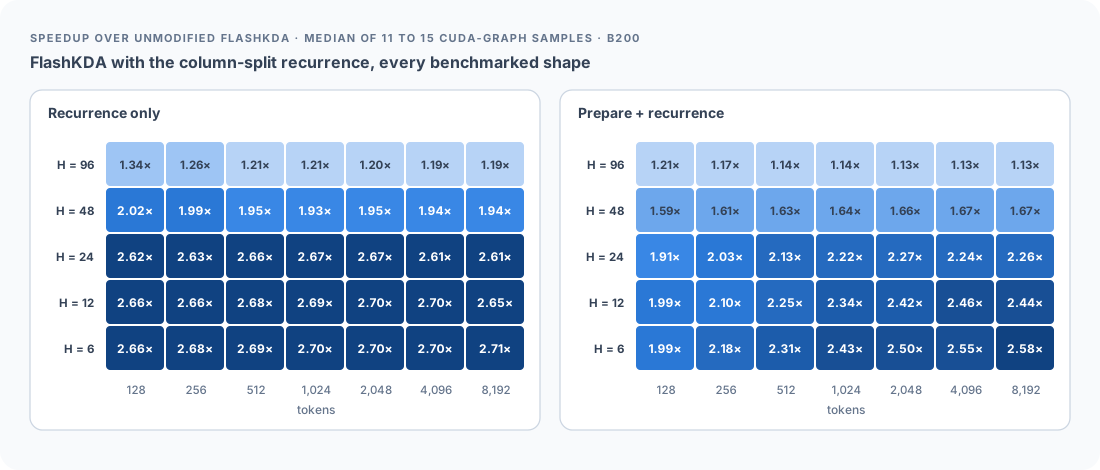
That flat line points to a GPU that is mostly idle, and this post is about filling it. We changed FlashKDA’s recurrence kernel so that one head’s state is spread across several SMs instead of one, and kept in registers instead of shared memory. The recurrence gets 2.6–2.7× faster for 24 heads or fewer, about 1.95× at 48 heads and 1.2× at 96. Both kernels together get up to 2.58× faster. Every output byte and every bit of the final state is identical to the original kernel’s.

1. FlashKDA in two kernels
For some background on KDA, read You Could Have Come Up With Kimi Delta Attention.
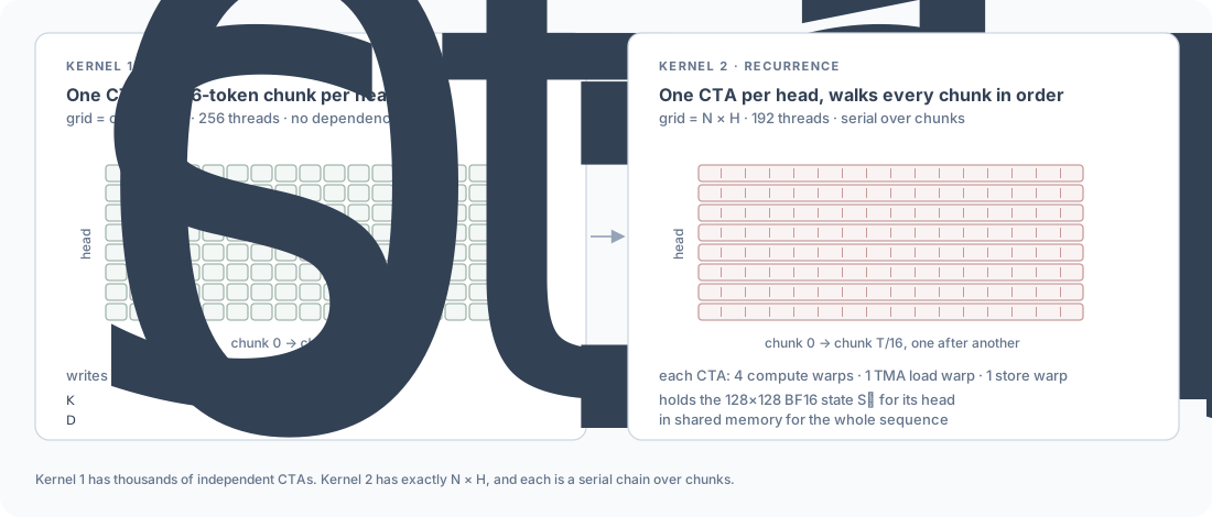
FlashKDA computes the chunkwise KDA forward pass over 16-token chunks in two kernels:
| Kernel | Grid | Threads per CTA | What it does |
|---|---|---|---|
| 1Prepare | chunks × heads | 256 |
|
| 2Recurrence | sequences × heads | 192 |
|
The first kernel is embarrassingly parallel. Every CTA handles one 16-token chunk of one head, so a long prompt launches thousands of CTAs. It writes a per-chunk workspace for the second kernel. Number the chunk’s tokens , let be token ‘s per-channel decay, and write for the decay from the start of the chunk to token . The workspace holds:
- and : each key and query decayed from the start of the chunk to its own token. Column is , or .
- : each key decayed from its own token to the end of the chunk. Row is .
- : the chunk’s total decay.
- : the inverse of a 16×16 lower-triangular matrix, where for measures how much token ‘s write disturbs token ‘s prediction.
- : the causal query-key scores, for .
The second kernel carries the recurrent state, which makes it the serial one. Each CTA loops over the entire set of tokens for a given Head and Batch pair, in chunks of 16 tokens. Your parallelism doesn’t grow with the number of chunks, so your only options for exposing parallelism is over heads and batches.
FlashKDA keeps the state entering chunk as a 128×128 BF16 matrix in shared memory, stored transposed as (keys by values). With the chunk’s values as the columns of , its outputs as the columns of and , for every chunk it computes:
Column of is token ‘s delta-rule error: what it writes into the state. These are the chunkwise equations derived in section 6 of the KDA post.
Each CTA has four compute warps, one warp issuing TMA loads into a three-stage ring, and one warp storing output tiles.
2. Where the time goes
Timing the two kernels separately shows the problem straight away:
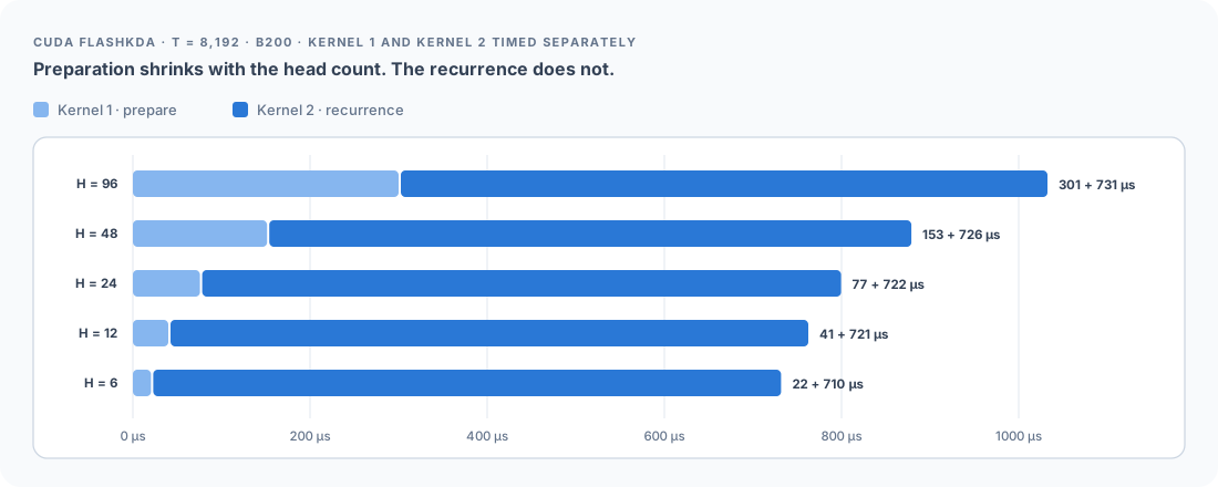
Preparation does sixteen times less work at 6 heads than at 96 and runs about fourteen times faster. The recurrence does sixteen times less work and runs at the same speed. At 6 heads it is 97% of the total.
The reason is the shape of its grid. One CTA per head means one SM per head. Each CTA walks 512 chunks one after another, and each chunk’s state update depends on the last. The run time is set by how long one head’s chain takes, not by how many heads there are. A B200 has 148 SMs:
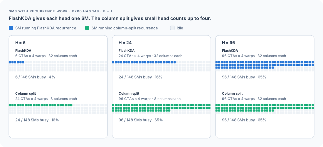
At 6 heads, 142 of the 148 SMs sit idle for the whole recurrence. If one head could be split across several SMs that idle hardware would be put to use.
3. Splitting the state
3.1 Every value column is independent
FlashKDA works in a transposed layout. It stores the state as , and the chunk’s values, errors and outputs as , and : one row per token, one column per value channel. Transposing the three per-chunk equations into that layout puts every per-chunk input on the left:

Follow value column (blue) through the chunk. Its column of gives its column of the prediction, which gives its column of , which gives its column of . Column (orange) takes the same path through the same shared inputs and never touches column . The output is built the same way as steps 1 and 2. So the value dimension splits into 128 independent recurrences that happen to share their inputs.
FlashKDA already uses this inside the CTA: each of its four compute warps owns 32 of the 128 columns. We apply the same split across SMs. A task becomes (sequence, head, slice of BV columns), and the grid becomes CTAs:
| Heads | BV | CTAs | SMs per head | Columns per warp |
|---|---|---|---|---|
| ≤ 24 | 32 | 4H | 4 | 8 |
| 48 | 64 | 96 | 2 | 16 |
| 96 | 128 | 96 | 1 | 32 (as in FlashKDA) |
We pick the smallest BV that keeps the grid at or below 148, so the kernel never launches more than one CTA per SM. Each CTA still has four compute warps, one per SM sub-partition, and a TMA loader warp. The preparation kernel and its workspace are unchanged.
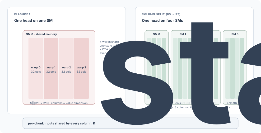
The slices share nothing they write, so the split needs no synchronization between CTAs at all: no flags, no atomics, no spinning. The only cost is that every slice CTA loads its own copy of the shared per-chunk inputs, up to four times as much input traffic. Those loads are small, served mostly from L2, and hidden behind the TMA pipeline.
3.2 Why more SMs is faster
Splitting doesn’t shorten the chain. Every chunk still has to wait for the one before it. What it changes is how many tensor cores work on each link of that chain at once.
In FlashKDA, one head’s whole state update runs on one SM. Each of its four compute warps owns 32 value columns, which is four 8-column MMA tiles, so every matrix multiply in a chunk is four HMMAs issued back to back on that SM’s tensor cores. Meanwhile, with 6 heads, the other 142 SMs and their tensor cores sit idle. They have nothing to do because the only remaining work is the next link of a chain that is still running somewhere else.
The column split puts those idle tensor cores to work. A head’s columns are spread over four SMs, and each warp owns just 8 columns, which is a single HMMA per matrix multiply. Sixteen warps on four SMs now share each chunk’s update instead of four warps on one, so four SMs’ worth of tensor cores work on the same link in parallel and the link finishes sooner.
This works because the recurrence is bound by latency, not throughput. In Nsight Compute the column-split kernel at 6 heads keeps the issue slots busy 5% of the time, with 0.35 eligible warps per scheduler. No single SM’s tensor cores are close to full. The limit is how long each link of the chain takes, so spreading a link over more tensor cores translates almost directly into wall-clock time:
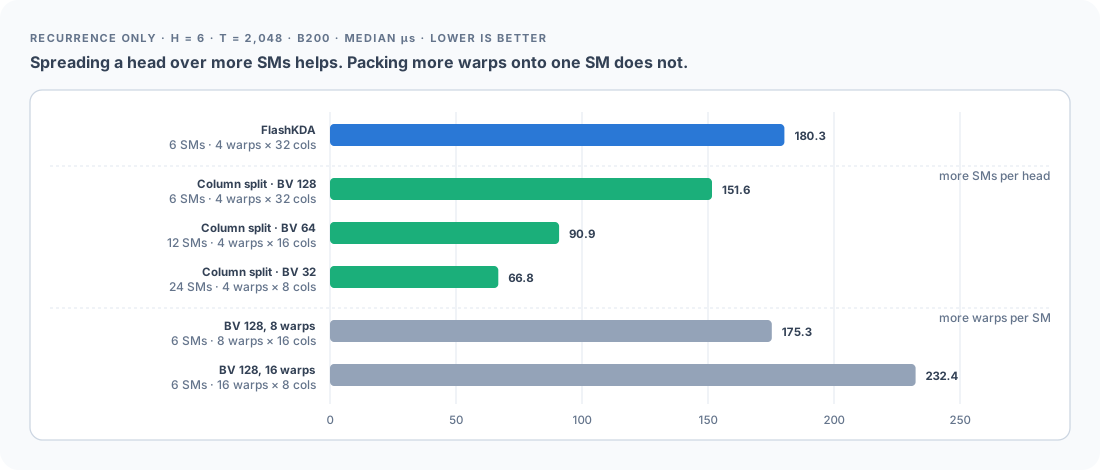
The bottom two bars are the control experiment. They give each warp the same 16 or 8 columns but keep all the warps for a head on one SM. That is barely better than FlashKDA, or worse. Every extra warp has to load the shared and operands from shared memory itself, and a single SM has a fixed number of tensor cores, schedulers and load paths to share between them. Spreading over SMs adds those resources; packing onto one SM only divides them.
3.3 Keeping the state in registers
The split has a second effect that matters even when it adds no SMs. Once a warp owns its columns outright, its state slice no longer needs to be in shared memory.
In FlashKDA the four warps share one buffer in shared memory. Each chunk, a warp loads its columns as MMA operands, computes the update and writes it back. Then all warps meet at a barrier before anyone reads the next chunk’s state. In the column-split kernel each warp keeps its slice in registers for the entire sequence. That is eight 16-row blocks in the MMA accumulator layout.
The one wrinkle is layout. The update produces the state in the MMA
accumulator layout, but the next chunk needs it as the MMA B-operand.
PTX’s movmatrix instruction transposes 8×8 tiles between the two inside a
warp’s registers, so the conversion never touches shared memory. Output tiles
also skip the staging buffer and store warp, and go straight from registers to
global memory.
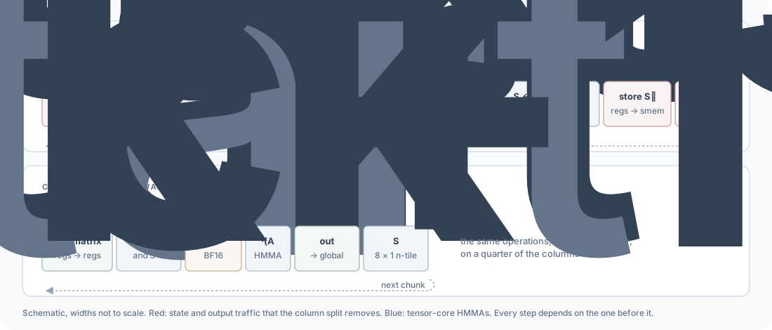
This is where the 1.2× at 96 heads comes from. There the column split uses BV = 128, the same 96 CTAs and 32 columns per warp as FlashKDA, so it gets no extra SMs. All of the gain comes from Figure 8: no state round trip, no barrier and a simpler output path.
3.4 Why the bits don’t change
FlashKDA is built with --use_fast_math, and its exact results depend on the
precise instruction behind every operation. We read those off the SASS of the
original build and kept every one of them in the modified kernel:
| Operation | Instruction in FlashKDA’s SASS |
|---|---|
| FP32 add, multiply, FMA | FADD.FTZ, FMUL.FTZ, FFMA.FTZ (denormals flushed) |
| BF16 arithmetic | HADD2.BF16, HMUL2.BF16, rounded once |
exp2, tanh | MUFU.EX2, MUFU.TANH |
| float → BF16 | F2FP, round to nearest |
| every matrix multiply | HMMA.16816.F32.BF16, in a fixed k-block order |
Per column, each warp runs the same m16n8k16 HMMA on the same k-blocks in the
same order. It applies the same FTZ FMA for the state update, the same BF16
subtract and multiply for , the same tanh-based sigmoid and BF16
rounding at the same points. Splitting by columns changes which warp computes
a column, never the order of any sum inside it. Every configuration we tried
(BV of 32, 64 and 128 with 4, 8 or 16 warps) is bitwise identical to FlashKDA.
3.5 What didn’t help
- Deeper pipelines. Three to eight input stages make no measurable difference; the loads are already hidden. (Going beyond four stages exposed a bug: a four-entry ring of release barriers aliased mbarrier phases and hung. The ring is now twice the stage count.)
- Offloading output work. A debug build that removed the entire output path saved only 7%, so dedicated output warps weren’t worth building.
- Overlapping the two kernels. The recurrence for chunk only needs the preparation output for chunk , so we tried running both kernels at once, synchronized by per-chunk ready flags. It was about 8% faster at 24 and 48 heads, but slower at 96 heads and at 12 or fewer, so we left it out.
What is left is the chain itself: 8 dependent HMMAs for
, the BF16 step, the
multiply, 8 HMMAs for the update,
the FMA and the movmatrix transpose, chunk after chunk. Reordering any of it
would change rounding, and with it the bits.
4. Results
All numbers are medians of 11 to 15 CUDA-graph samples per variant. Variants were sampled in rotating order, one exclusive B200 per head count, with compilation excluded. Both recurrence kernels read the same workspace written by FlashKDA’s preparation kernel. Before timing, the modified kernel’s output and final state were checked bitwise against FlashKDA’s in each of the 35 shapes.
The right-hand numbers add the preparation kernel’s time to each recurrence. Preparation is unchanged, so it costs the same in both columns.
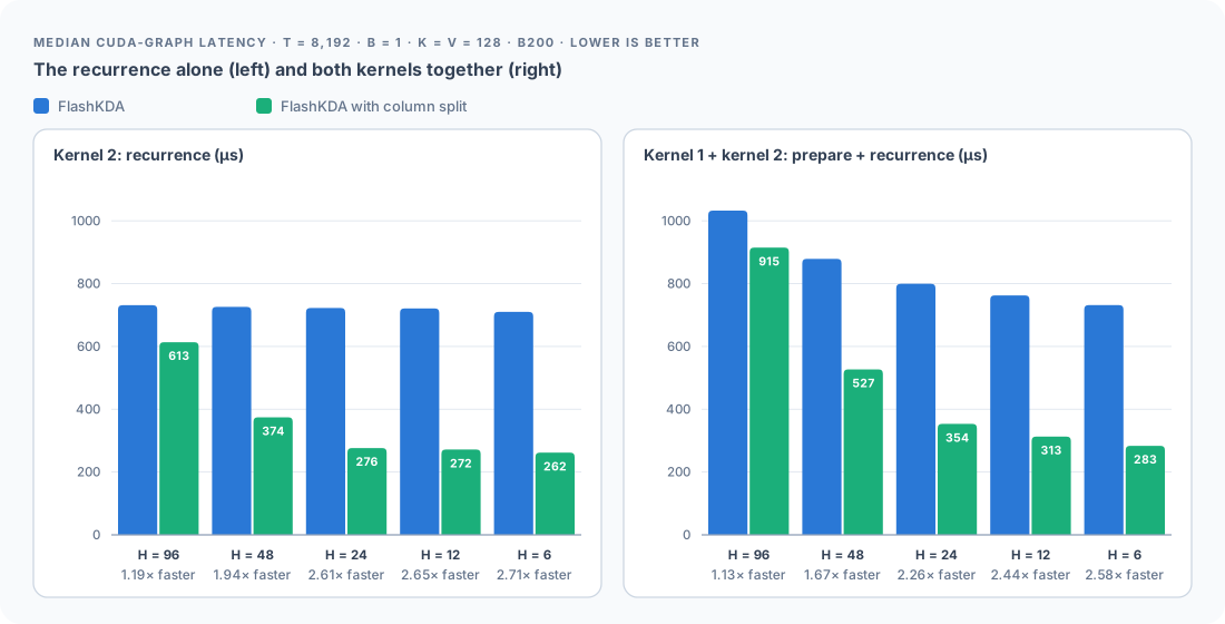
| Heads | Recurrence, FlashKDA (µs) | Recurrence, column split | Speedup | Both kernels, FlashKDA | Both kernels, column split | Speedup |
|---|---|---|---|---|---|---|
| 96 | 731.3 | 613.4 | 1.19× | 1032.6 | 914.7 | 1.13× |
| 48 | 726.1 | 374.2 | 1.94× | 878.8 | 526.9 | 1.67× |
| 24 | 722.5 | 276.5 | 2.61× | 799.5 | 353.5 | 2.26× |
| 12 | 721.2 | 271.8 | 2.65× | 762.5 | 313.1 | 2.44× |
| 6 | 710.0 | 261.7 | 2.71× | 731.7 | 283.4 | 2.58× |
The pattern holds at every sequence length we measured: